The independent distribution series of discrete random variables are given. Distribution law of a discrete random variable
Chapter 1. Discrete random variable
§ 1. Concepts of a random variable.
Distribution law of a discrete random variable.
Definition : Random is a quantity that, as a result of testing, takes only one value out of a possible set of its values, unknown in advance and depending on random reasons.
There are two types of random variables: discrete and continuous.
Definition : The random variable X is called discrete (discontinuous) if the set of its values is finite or infinite but countable.
In other words, the possible values of a discrete random variable can be renumbered.
A random variable can be described using its distribution law.
Definition : Distribution law of a discrete random variable call the correspondence between possible values of a random variable and their probabilities.
The distribution law of a discrete random variable X can be specified in the form of a table, in the first row of which all possible values of the random variable are indicated in ascending order, and in the second row the corresponding probabilities of these values, i.e.
where р1+ р2+…+ рn=1
Such a table is called a distribution series of a discrete random variable.
If the set of possible values of a random variable is infinite, then the series p1+ p2+…+ pn+… converges and its sum is equal to 1.
The distribution law of a discrete random variable X can be depicted graphically, for which a broken line is constructed in a rectangular coordinate system, connecting sequentially points with coordinates (xi; pi), i=1,2,…n. The resulting line is called distribution polygon (Fig. 1).
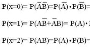
Organic chemistry" href="/text/category/organicheskaya_hiimya/" rel="bookmark">organic chemistry are 0.7 and 0.8, respectively. Draw up a distribution law for the random variable X - the number of exams that the student will pass.
Solution. The considered random variable X as a result of the exam can take one of the following values: x1=0, x2=1, x3=2.
Let's find the probability of these values. Let's denote the events:
https://pandia.ru/text/78/455/images/image004_81.jpg" width="259" height="66 src=">
 |
So, the distribution law of the random variable X is given by the table:
Control: 0.6+0.38+0.56=1.
§ 2. Distribution function
A complete description of a random variable is also given by the distribution function.
Definition: Distribution function of a discrete random variable X is called a function F(x), which determines for each value x the probability that the random variable X will take a value less than x:
F(x)=P(X<х)
Geometrically, the distribution function is interpreted as the probability that the random variable X will take the value that is represented on the number line by a point lying to the left of point x.
1)0≤ F(x) ≤1;
2) F(x) is a non-decreasing function on (-∞;+∞);
3) F(x) - continuous on the left at points x= xi (i=1,2,...n) and continuous at all other points;
4) F(-∞)=P (X<-∞)=0 как вероятность невозможного события Х<-∞,
F(+∞)=P(X<+∞)=1 как вероятность достоверного события Х<-∞.
If the distribution law of a discrete random variable X is given in the form of a table:
then the distribution function F(x) is determined by the formula:
https://pandia.ru/text/78/455/images/image007_76.gif" height="110">
0 for x≤ x1,
р1 at x1< х≤ x2,
F(x)= р1 + р2 at x2< х≤ х3
1 for x>xn.
Its graph is shown in Fig. 2:

§ 3. Numerical characteristics of a discrete random variable.
One of the important numerical characteristics is the mathematical expectation.
Definition: Mathematical expectation M(X) discrete random variable X is the sum of the products of all its values and their corresponding probabilities:
M(X) = ∑ xiрi= x1р1 + x2р2+…+ xnрn
The mathematical expectation serves as a characteristic of the average value of a random variable.
Properties of mathematical expectation:
1)M(C)=C, where C is a constant value;
2)M(C X)=C M(X),
3)M(X±Y)=M(X) ±M(Y);
4)M(X Y)=M(X) M(Y), where X, Y are independent random variables;
5)M(X±C)=M(X)±C, where C is a constant value;
To characterize the degree of dispersion of possible values of a discrete random variable around its mean value, dispersion is used.
Definition: Variance D ( X ) random variable X is the mathematical expectation of the squared deviation of the random variable from its mathematical expectation:
Dispersion properties:
1)D(C)=0, where C is a constant value;
2)D(X)>0, where X is a random variable;
3)D(C X)=C2 D(X), where C is a constant value;
4)D(X+Y)=D(X)+D(Y), where X, Y are independent random variables;
To calculate variance it is often convenient to use the formula:
D(X)=M(X2)-(M(X))2,
where M(X)=∑ xi2рi= x12р1 + x22р2+…+ xn2рn
The variance D(X) has the dimension of a squared random variable, which is not always convenient. Therefore, the value √D(X) is also used as an indicator of the dispersion of possible values of a random variable.
Definition: Standard deviation σ(X) random variable X is called the square root of the variance:
![]()
Task No. 2. The discrete random variable X is specified by the distribution law:
Find P2, the distribution function F(x) and plot its graph, as well as M(X), D(X), σ(X).
Solution: Since the sum of the probabilities of possible values of the random variable X is equal to 1, then
Р2=1- (0.1+0.3+0.2+0.3)=0.1
Let's find the distribution function F(x)=P(X Geometrically, this equality can be interpreted as follows: F(x) is the probability that the random variable will take the value that is represented on the number axis by a point lying to the left of point x. If x≤-1, then F(x)=0, since there is not a single value of this random variable on (-∞;x); If -1<х≤0, то F(х)=Р(Х=-1)=0,1, т. к. в промежуток (-∞;х) попадает только одно значение x1=-1; If 0<х≤1, то F(х)=Р(Х=-1)+ Р(Х=0)=0,1+0,1=0,2, т. к. в промежуток (-∞;x) there are two values x1=-1 and x2=0; If 1<х≤2, то F(х)=Р(Х=-1) + Р(Х=0)+ Р(Х=1)= 0,1+0,1+0,3=0,5, т. к. в промежуток (-∞;х) попадают три значения x1=-1, x2=0 и x3=1; If 2<х≤3, то F(х)=Р(Х=-1) + Р(Х=0)+ Р(Х=1)+ Р(Х=2)= 0,1+0,1+0,3+0,2=0,7, т. к. в промежуток (-∞;х) попадают четыре значения x1=-1, x2=0,x3=1 и х4=2; If x>3, then F(x)=P(X=-1) + P(X=0)+ P(X=1)+ P(X=2)+P(X=3)= 0.1 +0.1+0.3+0.2+0.3=1, because four values x1=-1, x2=0, x3=1, x4=2 fall into the interval (-∞;x) and x5=3. https://pandia.ru/text/78/455/images/image006_89.gif" width="14 height=2" height="2"> 0 at x≤-1, 0.1 at -1<х≤0, 0.2 at 0<х≤1, F(x)= 0.5 at 1<х≤2, 0.7 at 2<х≤3, 1 at x>3 Let's represent the function F(x) graphically (Fig. 3): https://pandia.ru/text/78/455/images/image014_24.jpg" width="158 height=29" height="29">≈1.2845. §
4. Binomial distribution law discrete random variable, Poisson's law. Definition: Binomial
is called the law of distribution of a discrete random variable X - the number of occurrences of event A in n independent repeated trials, in each of which event A may occur with probability p or not occur with probability q = 1-p. Then P(X=m) - the probability of occurrence of event A exactly m times in n trials is calculated using the Bernoulli formula: Р(Х=m)=Сmnpmqn-m The mathematical expectation, dispersion and standard deviation of a random variable X distributed according to a binary law are found, respectively, using the formulas: https://pandia.ru/text/78/455/images/image016_31.gif" width="26"> The probability of event A - “rolling out a five” in each trial is the same and equal to 1/6, i.e. . P(A)=p=1/6, then P(A)=1-p=q=5/6, where - “failure to get an A.” The random variable X can take the following values: 0;1;2;3. We find the probability of each of the possible values of X using Bernoulli’s formula: Р(Х=0)=Р3(0)=С03р0q3=1 (1/6)0 (5/6)3=125/216; Р(Х=1)=Р3(1)=С13р1q2=3 (1/6)1 (5/6)2=75/216; Р(Х=2)=Р3(2)=С23р2q =3 (1/6)2 (5/6)1=15/216; Р(Х=3)=Р3(3)=С33р3q0=1 (1/6)3 (5/6)0=1/216. That. the distribution law of the random variable X has the form: Control: 125/216+75/216+15/216+1/216=1. Let's find the numerical characteristics of the random variable X: M(X)=np=3 (1/6)=1/2, D(X)=npq=3 (1/6) (5/6)=5/12, Task No. 4. An automatic machine stamps parts. The probability that a manufactured part will be defective is 0.002. Find the probability that among 1000 selected parts there will be: a) 5 defective; b) at least one is defective. Solution:
The number n=1000 is large, the probability of producing a defective part p=0.002 is small, and the events under consideration (the part turns out to be defective) are independent, therefore the Poisson formula holds: Рn(m)= e-
λ
λm Let's find λ=np=1000 0.002=2. a) Find the probability that there will be 5 defective parts (m=5): Р1000(5)= e-2
25
= 32 0,13534
= 0,0361 b) Find the probability that there will be at least one defective part. Event A - “at least one of the selected parts is defective” is the opposite of the event - “all selected parts are not defective.” Therefore, P(A) = 1-P(). Hence the desired probability is equal to: P(A)=1-P1000(0)=1- e-2
20
= 1- e-2=1-0.13534≈0.865. Tasks for independent work.
1.1
1.2.
The dispersed random variable X is specified by the distribution law: Find p4, the distribution function F(X) and plot its graph, as well as M(X), D(X), σ(X). 1.3.
There are 9 markers in the box, 2 of which no longer write. Take 3 markers at random. Random variable X is the number of writing markers among those taken. Draw up a law of distribution of a random variable. 1.4.
There are 6 textbooks randomly arranged on a library shelf, 4 of which are bound. The librarian takes 4 textbooks at random. Random variable X is the number of bound textbooks among those taken. Draw up a law of distribution of a random variable. 1.5.
There are two tasks on the ticket. The probability of correctly solving the first problem is 0.9, the second is 0.7. Random variable X is the number of correctly solved problems in the ticket. Draw up a distribution law, calculate the mathematical expectation and variance of this random variable, and also find the distribution function F(x) and build its graph. 1.6.
Three shooters are shooting at a target. The probability of hitting the target with one shot is 0.5 for the first shooter, 0.8 for the second, and 0.7 for the third. Random variable X is the number of hits on the target if the shooters fire one shot at a time. Find the distribution law, M(X),D(X). 1.7.
A basketball player throws the ball into the basket with a probability of hitting each shot of 0.8. For each hit, he receives 10 points, and if he misses, no points are awarded to him. Draw up a distribution law for the random variable X - the number of points received by a basketball player in 3 shots. Find M(X),D(X), as well as the probability that he gets more than 10 points. 1.8.
Letters are written on the cards, a total of 5 vowels and 3 consonants. 3 cards are chosen at random, and each time the taken card is returned back. Random variable X is the number of vowels among those taken. Draw up a distribution law and find M(X),D(X),σ(X). 1.9.
On average, under 60% of contracts, the insurance company pays insurance amounts in connection with the occurrence of an insured event. Draw up a distribution law for the random variable X - the number of contracts for which the insurance amount was paid among four contracts selected at random. Find the numerical characteristics of this quantity. 1.10.
The radio station sends call signs (no more than four) at certain intervals until two-way communication is established. The probability of receiving a response to a call sign is 0.3. Random variable X is the number of call signs sent. Draw up a distribution law and find F(x). 1.11.
There are 3 keys, of which only one fits the lock. Draw up a law for the distribution of the random variable X-number of attempts to open the lock, if the tried key does not participate in subsequent attempts. Find M(X),D(X). 1.12.
Consecutive independent tests of three devices are carried out for reliability. Each subsequent device is tested only if the previous one turned out to be reliable. The probability of passing the test for each device is 0.9. Draw up a distribution law for the random variable X-number of tested devices. 1.13
.Discrete random variable X has three possible values: x1=1, x2, x3, and x1<х2<х3. Вероятность того, что Х примет значения х1 и х2, соответственно равны 0,3 и 0,2. Известно, что М(Х)=2,2, D(X)=0,76. Составить закон распределения случайной величины. 1.14.
The electronic device block contains 100 identical elements. The probability of failure of each element during time T is 0.002. The elements work independently. Find the probability that no more than two elements will fail during time T. 1.15.
The textbook was published in a circulation of 50,000 copies. The probability that the textbook is bound incorrectly is 0.0002. Find the probability that the circulation contains: a) four defective books, b) less than two defective books. 1
.16.
The number of calls arriving at the PBX every minute is distributed according to Poisson's law with the parameter λ=1.5. Find the probability that in a minute the following will arrive: a) two calls; b) at least one call. 1.17.
Find M(Z),D(Z) if Z=3X+Y. 1.18.
The laws of distribution of two independent random variables are given: Find M(Z),D(Z) if Z=X+2Y. Answers:
https://pandia.ru/text/78/455/images/image007_76.gif" height="110"> 1.1.
p3=0.4; 0 at x≤-2, 0.3 at -2<х≤0, F(x)= 0.5 at 0<х≤2, 0.9 at 2<х≤5, 1 at x>5 0.3 at -1<х≤0, 0.4 at 0<х≤1, F(x)= 0.6 at 1<х≤2, 0.7 at 2<х≤3, 1 at x>3 M(X)=1; D(X)=2.6; σ(X) ≈1.612. https://pandia.ru/text/78/455/images/image025_24.gif" width="2 height=98" height="98"> 0 at x≤0, 0.03 at 0<х≤1, F(x)= 0.37 at 1<х≤2, 1 for x>2 M(X)=2; D(X)=0.62 M(X)=2.4; D(X)=0.48, P(X>10)=0.896 1.
8
.
M(X)=15/8; D(X)=45/64; σ(X) ≈ M(X)=2.4; D(X)=0.96 https://pandia.ru/text/78/455/images/image008_71.gif" width="14"> 1.11.
M(X)=2; D(X)=2/3 1.14.
1.22 e-0.2≈0.999 1.15.
a)0.0189; b) 0.00049 1.16.
a)0.0702; b)0.77687 1.17.
3,8; 14,2 1.18.
11,2; 4. Chapter 2. Continuous random variable
Definition: Continuous
is a quantity whose all possible values completely fill a finite or infinite span of the number line. Obviously, the number of possible values of a continuous random variable is infinite. A continuous random variable can be specified using a distribution function. Definition: F distribution function
a continuous random variable X is called a function F(x), which determines for each value xhttps://pandia.ru/text/78/455/images/image028_11.jpg" width="14" height="13">R The distribution function is sometimes called the cumulative distribution function. Properties of the distribution function:
1)1≤ F(x) ≤1 2) For a continuous random variable, the distribution function is continuous at any point and differentiable everywhere, except, perhaps, at individual points. 3) The probability of a random variable X falling into one of the intervals (a;b), [a;b], [a;b], is equal to the difference between the values of the function F(x) at points a and b, i.e. R(a)<Х 4) The probability that a continuous random variable X will take one separate value is 0. 5) F(-∞)=0, F(+∞)=1 Specifying a continuous random variable using a distribution function is not the only way. Let us introduce the concept of probability distribution density (distribution density). Definition
:
Probability distribution density
f
(
x
)
of a continuous random variable X is the derivative of its distribution function, i.e.: The probability density function is sometimes called the differential distribution function or differential distribution law. The graph of the probability density distribution f(x) is called probability distribution curve
.
Properties of probability density distribution:
1) f(x) ≥0, at xhttps://pandia.ru/text/78/455/images/image029_10.jpg" width="285" height="141">DIV_ADBLOCK13"> https://pandia.ru/text/78/455/images/image032_23.gif" height="38 src="> +∞ 2 6 +∞ 6 6 ∫ f(x)dx=∫ 0dx+ ∫ c(x-2)dx +∫ 0dx= c∫ (x-2)dx=c(x2/2-2x) =c(36/2-12-(4/ 2-4))=8s; b) It is known that F(x)= ∫ f(x)dx Therefore, x if x≤2, then F(x)= ∫ 0dx=0; https://pandia.ru/text/78/455/images/image032_23.gif" height="38 src="> 2 6 x 6 6 if x>6, then F(x)= ∫ 0dx+∫ 1/8(x-2)dx+∫ 0dx=1/8∫(x-2)dx=1/8(x2/2-2x) = 1/8(36/2-12-(4/2+4))=1/8 8=1. Thus, 0 at x≤2, F(x)= (x-2)2/16 at 2<х≤6, 1 for x>6. The graph of the function F(x) is shown in Fig. 3 https://pandia.ru/text/78/455/images/image034_23.gif" width="14" height="62 src="> 0 at x≤0, F(x)= (3 arctan x)/π at 0<х≤√3, 1 for x>√3. Find the differential distribution function f(x) Solution:
Since f(x)= F’(x), then DIV_ADBLOCK14"> · Mathematical expectation M (X)
continuous random variable X are determined by the equality: M(X)= ∫ x f(x)dx, provided that this integral converges absolutely. · Dispersion
D
(
X
)
continuous random variable X is determined by the equality: D(X)= ∫ (x-M(x)2) f(x)dx, or D(X)= ∫ x2 f(x)dx - (M(x))2 · Standard deviation σ(X)
continuous random variable is determined by the equality: All properties of mathematical expectation and dispersion, discussed earlier for dispersed random variables, are also valid for continuous ones. Task No. 3. The random variable X is specified by the differential function f(x): https://pandia.ru/text/78/455/images/image036_19.gif" height="38"> -∞ 2 X3/9 + x2/6 = 8/9-0+9/6-4/6=31/18, https://pandia.ru/text/78/455/images/image032_23.gif" height="38"> +∞ D(X)= ∫ x2 f(x)dx-(M(x))2=∫ x2 x/3 dx+∫1/3x2 dx=(31/18)2=x4/12 + x3/9 - - (31/18)2=16/12-0+27/9-8/9-(31/18)2=31/9- (31/18)2==31/9(1-31/36)=155/324, https://pandia.ru/text/78/455/images/image032_23.gif" height="38"> P(1<х<5)= ∫ f(x)dx=∫ х/3 dx+∫ 1/3 dx+∫ 0 dx= х2/6 +1/3х = 4/6-1/6+1-2/3=5/6. Problems for independent solution.
2.1.
A continuous random variable X is specified by the distribution function: 0 at x≤0, F(x)= https://pandia.ru/text/78/455/images/image038_17.gif" width="14" height="86"> 0 for x≤ π/6, F(x)= - cos 3x at π/6<х≤ π/3, 1 for x> π/3. Find the differential distribution function f(x), and also Р(2π /9<Х< π /2). 2.3.
0 at x≤2, f(x)= c x at 2<х≤4, 0 for x>4. 2.4.
A continuous random variable X is specified by the distribution density: 0 at x≤0, f(x)= c √x at 0<х≤1, 0 for x>1. Find: a) number c; b) M(X), D(X). 2.5.
https://pandia.ru/text/78/455/images/image041_3.jpg" width="36" height="39"> at x, 0 at x. Find: a) F(x) and construct its graph; b) M(X),D(X), σ(X); c) the probability that in four independent trials the value of X will take exactly 2 times the value belonging to the interval (1;4). 2.6.
The probability distribution density of a continuous random variable X is given: f(x)= 2(x-2) at x, 0 at x. Find: a) F(x) and plot it; b) M(X),D(X), σ (X); c) the probability that in three independent trials the value of X will take exactly 2 times the value belonging to the segment . 2.7.
The function f(x) is given as: https://pandia.ru/text/78/455/images/image045_4.jpg" width="43" height="38 src=">.jpg" width="16" height="15">[-√ 3/2; √3/2]. 2.8.
The function f(x) is given as: https://pandia.ru/text/78/455/images/image046_5.jpg" width="45" height="36 src="> .jpg" width="16" height="15">[- π /4 ; π /4]. Find: a) the value of the constant c at which the function will be the probability density of some random variable X; b) distribution function F(x). 2.9.
The random variable X, concentrated on the interval (3;7), is specified by the distribution function F(x)= . Find the probability that random variable X will take the value: a) less than 5, b) not less than 7. 2.10.
Random variable X, concentrated on the interval (-1;4), is given by the distribution function F(x)= . Find the probability that random variable X will take the value: a) less than 2, b) not less than 4. 2.11.
https://pandia.ru/text/78/455/images/image049_6.jpg" width="43" height="44 src="> .jpg" width="16" height="15">. Find: a) number c; b) M(X); c) probability P(X> M(X)). 2.12.
The random variable is specified by the differential distribution function: https://pandia.ru/text/78/455/images/image050_3.jpg" width="60" height="38 src=">.jpg" width="16 height=15" height="15"> . Find: a) M(X); b) probability P(X≤M(X)) 2.13.
The Rem distribution is given by the probability density: https://pandia.ru/text/78/455/images/image052_5.jpg" width="46" height="37"> for x ≥0. Prove that f(x) is indeed a probability density function. 2.14.
The probability distribution density of a continuous random variable X is given: DIV_ADBLOCK17"> https://pandia.ru/text/78/455/images/image055_3.jpg" width="187 height=136" height="136">(Fig. 5) 2.16.
The random variable X is distributed according to the “right triangle” law in the interval (0;4) (Fig. 5). Find an analytical expression for the probability density f(x) on the entire number line. Answers
0 at x≤0, f(x)= https://pandia.ru/text/78/455/images/image038_17.gif" width="14" height="86"> 0 for x≤ π/6, F(x)= 3sin 3x at π/6<х≤ π/3,
Непрерывная случайная величина Х имеет равномерный закон распределения на некотором интервале (а;b), которому принадлежат все возможные значения Х, если плотность распределения вероятностей f(x) постоянная на этом интервале и равна 0 вне его, т. е. 0 for x≤a, f(x)= for a<х 0 for x≥b. The graph of the function f(x) is shown in Fig. 1 F(x)= https://pandia.ru/text/78/455/images/image077_3.jpg" width="30" height="37">, D(X)=, σ(X)=. Task No. 1. The random variable X is uniformly distributed on the segment. Find: a) probability distribution density f(x) and plot it; b) the distribution function F(x) and plot it; c) M(X),D(X), σ(X). Solution:
Using the formulas discussed above, with a=3, b=7, we find: https://pandia.ru/text/78/455/images/image081_2.jpg" width="22" height="39"> at 3≤х≤7, 0 for x>7 Let's build its graph (Fig. 3): https://pandia.ru/text/78/455/images/image038_17.gif" width="14" height="86 src="> 0 at x≤3, F(x)= https://pandia.ru/text/78/455/images/image084_3.jpg" width="203" height="119 src=">Fig. 4 D(X) = ==https://pandia.ru/text/78/455/images/image089_1.jpg" width="37" height="43">==https://pandia.ru/text/ 78/455/images/image092_10.gif" width="14" height="49 src="> 0 at x<0, f(x)= λе-λх for x≥0. The distribution function of a random variable X, distributed according to the exponential law, is given by the formula: DIV_ADBLOCK19"> https://pandia.ru/text/78/455/images/image095_4.jpg" width="161" height="119 src="> Fig. 6 The mathematical expectation, variance and standard deviation of the exponential distribution are respectively equal to: M(X)= , D(X)=, σ (Х)= Thus, the mathematical expectation and the standard deviation of the exponential distribution are equal to each other. The probability of X falling into the interval (a;b) is calculated by the formula: P(a<Х Task No. 2. The average failure-free operation time of the device is 100 hours. Assuming that the failure-free operation time of the device has an exponential distribution law, find: a) probability distribution density; b) distribution function; c) the probability that the device’s failure-free operation time will exceed 120 hours. Solution:
According to the condition, the mathematical distribution M(X)=https://pandia.ru/text/78/455/images/image098_10.gif" height="43 src="> 0 at x<0, a) f(x)= 0.01e -0.01x for x≥0. b) F(x)= 0 at x<0, 1-e -0.01x at x≥0. c) We find the desired probability using the distribution function: P(X>120)=1-F(120)=1-(1- e -1.2)= e -1.2≈0.3. §
3.Normal distribution law Definition:
A continuous random variable X has normal distribution law (Gauss's law),
if its distribution density has the form: where m=M(X), σ2=D(X), σ>0. The normal distribution curve is called normal or Gaussian curve
(Fig.7) The distribution function of a random variable X, distributed according to the normal law, is expressed through the Laplace function Ф (x) according to the formula: where is the Laplace function. Comment:
The function Ф(x) is odd (Ф(-х)=-Ф(х)), in addition, for x>5 we can assume Ф(х) ≈1/2. The graph of the distribution function F(x) is shown in Fig. 8 https://pandia.ru/text/78/455/images/image106_4.jpg" width="218" height="33"> The probability that the absolute value of the deviation is less than a positive number δ is calculated by the formula: In particular, for m=0 the following equality holds: "Three Sigma Rule"
If a random variable X has a normal distribution law with parameters m and σ, then it is almost certain that its value lies in the interval (a-3σ; a+3σ), because https://pandia.ru/text/78/455/images/image110_2.jpg" width="157" height="57 src=">a) b) Let's use the formula: https://pandia.ru/text/78/455/images/image112_2.jpg" width="369" height="38 src="> From the table of function values Ф(х) we find Ф(1.5)=0.4332, Ф(1)=0.3413. So, the desired probability: P(28 Tasks for independent work
3.1.
The random variable X is uniformly distributed in the interval (-3;5). Find: b) distribution function F(x); c) numerical characteristics; d) probability P(4<х<6). 3.2.
The random variable X is uniformly distributed on the segment. Find: a) distribution density f(x); b) distribution function F(x); c) numerical characteristics; d) probability P(3≤х≤6). 3.3.
An automatic traffic light is installed on the highway, in which the green light is on for 2 minutes for vehicles, yellow for 3 seconds and red for 30 seconds, etc. A car drives along the highway at a random moment in time. Find the probability that a car will pass a traffic light without stopping. 3.4.
Subway trains run regularly at intervals of 2 minutes. A passenger enters the platform at a random time. What is the probability that a passenger will have to wait more than 50 seconds for a train? Find the mathematical expectation of the random variable X - the waiting time for the train. 3.5.
Find the variance and standard deviation of the exponential distribution given by the distribution function: F(x)= 0 at x<0, 1st-8x for x≥0. 3.6.
A continuous random variable X is specified by the probability distribution density: f(x)= 0 at x<0, 0.7 e-0.7x at x≥0. a) Name the distribution law of the random variable under consideration. b) Find the distribution function F(X) and the numerical characteristics of the random variable X. 3.7.
The random variable X is distributed according to the exponential law specified by the probability distribution density: f(x)= 0 at x<0, 0.4 e-0.4 x at x≥0. Find the probability that as a result of the test X will take a value from the interval (2.5;5). 3.8.
A continuous random variable X is distributed according to the exponential law specified by the distribution function: F(x)= 0 at x<0, 1st-0.6x at x≥0 Find the probability that, as a result of the test, X will take a value from the segment. 3.9.
The expected value and standard deviation of a normally distributed random variable are 8 and 2, respectively. Find: a) distribution density f(x); b) the probability that as a result of the test X will take a value from the interval (10;14). 3.10.
The random variable X is normally distributed with a mathematical expectation of 3.5 and a variance of 0.04. Find: a) distribution density f(x); b) the probability that as a result of the test X will take a value from the segment . 3.11.
The random variable X is normally distributed with M(X)=0 and D(X)=1. Which of the events: |X|≤0.6 or |X|≥0.6 is more likely? 3.12.
The random variable X is distributed normally with M(X)=0 and D(X)=1. From which interval (-0.5;-0.1) or (1;2) is it more likely to take a value during one test? 3.13.
The current price per share can be modeled using the normal distribution law with M(X)=10 den. units and σ (X)=0.3 den. units Find: a) the probability that the current share price will be from 9.8 den. units up to 10.4 days units; b) using the “three sigma rule”, find the boundaries within which the current stock price will be located. 3.14.
The substance is weighed without systematic errors. Random weighing errors are subject to the normal law with the mean square ratio σ=5g. Find the probability that in four independent experiments an error in three weighings will not occur in absolute value 3r. 3.15.
The random variable X is normally distributed with M(X)=12.6. The probability of a random variable falling into the interval (11.4;13.8) is 0.6826. Find the standard deviation σ. 3.16.
The random variable X is distributed normally with M(X)=12 and D(X)=36. Find the interval into which the random variable X will fall as a result of the test with a probability of 0.9973. 3.17.
A part manufactured by an automatic machine is considered defective if the deviation X of its controlled parameter from the nominal value exceeds modulo 2 units of measurement. It is assumed that the random variable X is normally distributed with M(X)=0 and σ(X)=0.7. What percentage of defective parts does the machine produce? 3.18.
The X parameter of the part is distributed normally with a mathematical expectation of 2 equal to the nominal value and a standard deviation of 0.014. Find the probability that the deviation of X from the nominal value will not exceed 1% of the nominal value. Answers
https://pandia.ru/text/78/455/images/image116_9.gif" width="14" height="110 src="> b) 0 for x≤-3, F(x)= left"> 3.10.
a)f(x)= , b) Р(3.1≤Х≤3.7) ≈0.8185. 3.11.
|x|≥0.6. 3.12.
(-0,5;-0,1). 3.13.
a) P(9.8≤Х≤10.4) ≈0.6562. 3.14.
0,111. 3.15.
σ=1.2. 3.16.
(-6;30). 3.17.
0,4%. Random variable A variable is called a variable that, as a result of each test, takes on one previously unknown value, depending on random reasons. Random variables are denoted by capital Latin letters: $X,\ Y,\ Z,\ \dots $ According to their type, random variables can be discrete And continuous. Discrete random variable- this is a random variable whose values can be no more than countable, that is, either finite or countable. By countability we mean that the values of a random variable can be numbered. Example 1
. Here are examples of discrete random variables: a) the number of hits on the target with $n$ shots, here the possible values are $0,\ 1,\ \dots ,\ n$. b) the number of emblems dropped when tossing a coin, here the possible values are $0,\ 1,\ \dots ,\ n$. c) the number of ships arriving on board (a countable set of values). d) the number of calls arriving at the PBX (countable set of values). A discrete random variable $X$ can take values $x_1,\dots ,\ x_n$ with probabilities $p\left(x_1\right),\ \dots ,\ p\left(x_n\right)$. The correspondence between these values and their probabilities is called law of distribution of a discrete random variable. As a rule, this correspondence is specified using a table, the first line of which indicates the values $x_1,\dots ,\ x_n$, and the second line contains the probabilities $p_1,\dots ,\ p_n$ corresponding to these values. $\begin(array)(|c|c|) Example 2
. Let the random variable $X$ be the number of points rolled when tossing a die. Such a random variable $X$ can take the following values: $1,\ 2,\ 3,\ 4,\ 5,\ 6$. The probabilities of all these values are equal to $1/6$. Then the law of probability distribution of the random variable $X$: $\begin(array)(|c|c|) Comment. Since in the distribution law of a discrete random variable $X$ the events $1,\ 2,\ \dots ,\ 6$ form a complete group of events, then the sum of the probabilities must be equal to one, that is, $\sum(p_i)=1$. Expectation of a random variable sets its “central” meaning. For a discrete random variable, the mathematical expectation is calculated as the sum of the products of the values $x_1,\dots ,\ x_n$ and the probabilities $p_1,\dots ,\ p_n$ corresponding to these values, that is: $M\left(X\right)=\sum ^n_(i=1)(p_ix_i)$. In English-language literature, another notation $E\left(X\right)$ is used. Properties of mathematical expectation$M\left(X\right)$: Example 3
. Let's find the mathematical expectation of the random variable $X$ from example $2$. $$M\left(X\right)=\sum^n_(i=1)(p_ix_i)=1\cdot ((1)\over (6))+2\cdot ((1)\over (6) )+3\cdot ((1)\over (6))+4\cdot ((1)\over (6))+5\cdot ((1)\over (6))+6\cdot ((1 )\over (6))=3.5.$$ We can notice that $M\left(X\right)$ lies between the smallest ($1$) and largest ($6$) values of the random variable $X$. Example 4
. It is known that the mathematical expectation of the random variable $X$ is equal to $M\left(X\right)=2$. Find the mathematical expectation of the random variable $3X+5$. Using the above properties, we get $M\left(3X+5\right)=M\left(3X\right)+M\left(5\right)=3M\left(X\right)+5=3\cdot 2 +5=$11. Example 5
. It is known that the mathematical expectation of the random variable $X$ is equal to $M\left(X\right)=4$. Find the mathematical expectation of the random variable $2X-9$. Using the above properties, we get $M\left(2X-9\right)=M\left(2X\right)-M\left(9\right)=2M\left(X\right)-9=2\cdot 4 -9=-1$. Possible values of random variables with equal mathematical expectations can disperse differently around their average values. For example, in two student groups the average score for the exam in probability theory turned out to be 4, but in one group everyone turned out to be good students, and in the other group there were only C students and excellent students. Therefore, there is a need for a numerical characteristic of a random variable that would show the spread of the values of the random variable around its mathematical expectation. This characteristic is dispersion. Variance of a discrete random variable$X$ is equal to: $$D\left(X\right)=\sum^n_(i=1)(p_i(\left(x_i-M\left(X\right)\right))^2).\ $$ In English literature the notation $V\left(X\right),\ Var\left(X\right)$ is used. Very often the variance $D\left(X\right)$ is calculated using the formula $D\left(X\right)=\sum^n_(i=1)(p_ix^2_i)-(\left(M\left(X \right)\right))^2$. Dispersion properties$D\left(X\right)$: Example 6
. Let's calculate the variance of the random variable $X$ from example $2$. $$D\left(X\right)=\sum^n_(i=1)(p_i(\left(x_i-M\left(X\right)\right))^2)=((1)\over (6))\cdot (\left(1-3.5\right))^2+((1)\over (6))\cdot (\left(2-3.5\right))^2+ \dots +((1)\over (6))\cdot (\left(6-3.5\right))^2=((35)\over (12))\approx 2.92.$$ Example 7
. It is known that the variance of the random variable $X$ is equal to $D\left(X\right)=2$. Find the variance of the random variable $4X+1$. Using the above properties, we find $D\left(4X+1\right)=D\left(4X\right)+D\left(1\right)=4^2D\left(X\right)+0=16D\ left(X\right)=16\cdot 2=32$. Example 8
. It is known that the variance of the random variable $X$ is equal to $D\left(X\right)=3$. Find the variance of the random variable $3-2X$. Using the above properties, we find $D\left(3-2X\right)=D\left(3\right)+D\left(2X\right)=0+2^2D\left(X\right)=4D\ left(X\right)=4\cdot 3=12$. The method of representing a discrete random variable in the form of a distribution series is not the only one, and most importantly, it is not universal, since a continuous random variable cannot be specified using a distribution series. There is another way to represent a random variable - the distribution function. Distribution function random variable $X$ is called a function $F\left(x\right)$, which determines the probability that the random variable $X$ will take a value less than some fixed value $x$, that is, $F\left(x\right )=P\left(X< x\right)$ Properties of the distribution function: Example 9
. Let us find the distribution function $F\left(x\right)$ for the distribution law of the discrete random variable $X$ from example $2$. $\begin(array)(|c|c|) If $x\le 1$, then, obviously, $F\left(x\right)=0$ (including for $x=1$ $F\left(1\right)=P\left(X< 1\right)=0$). If $1< x\le 2$, то $F\left(x\right)=P\left(X=1\right)=1/6$. If $2< x\le 3$, то $F\left(x\right)=P\left(X=1\right)+P\left(X=2\right)=1/6+1/6=1/3$. If $3< x\le 4$, то $F\left(x\right)=P\left(X=1\right)+P\left(X=2\right)+P\left(X=3\right)=1/6+1/6+1/6=1/2$. If $4< x\le 5$, то $F\left(X\right)=P\left(X=1\right)+P\left(X=2\right)+P\left(X=3\right)+P\left(X=4\right)=1/6+1/6+1/6+1/6=2/3$. If $5< x\le 6$, то $F\left(x\right)=P\left(X=1\right)+P\left(X=2\right)+P\left(X=3\right)+P\left(X=4\right)+P\left(X=5\right)=1/6+1/6+1/6+1/6+1/6=5/6$. If $x > 6$, then $F\left(x\right)=P\left(X=1\right)+P\left(X=2\right)+P\left(X=3\right) +P\left(X=4\right)+P\left(X=5\right)+P\left(X=6\right)=1/6+1/6+1/6+1/6+ 1/6+1/6=1$. So $F(x)=\left\(\begin(matrix) Definition 1 A random variable $X$ is called discrete (discontinuous) if the set of its values is infinite or finite but countable. In other words, a quantity is called discrete if its values can be numbered. A random variable can be described using the distribution law. The distribution law of a discrete random variable $X$ can be specified in the form of a table, the first line of which indicates all possible values of the random variable in ascending order, and the second line contains the corresponding probabilities of these values: Figure 1. where $р1+ р2+ ... + рn = 1$. This table is near the distribution of a discrete random variable. If the set of possible values of a random variable is infinite, then the series $р1+ р2+ ... + рn+ ...$ converges and its sum will be equal to $1$. The distribution law of a discrete random variable $X$ can be represented graphically, for which a broken line is constructed in the coordinate system (rectangular), which sequentially connects points with coordinates $(xi;pi), i=1,2, ... n$. The line we got is called distribution polygon. Figure 2. The distribution law of a discrete random variable $X$ can also be represented analytically (using the formula): $P(X=xi)= \varphi (xi),i =1,2,3 ... n$. When solving many problems in probability theory, it is necessary to carry out operations of multiplying a discrete random variable by a constant, adding two random variables, multiplying them, substituting them to a power. In these cases, it is necessary to adhere to the following rules for random discrete quantities: Definition 3 Multiplication of a discrete random variable $X$ by a constant $K$ is a discrete random variable $Y=KX,$ which is determined by the equalities: $y_i=Kx_i,\ \ p\left(y_i\right)=p\left(x_i\right)= p_i,\ \ i=\overline(1,\ n).$ Definition 4 Two random variables $x$ and $y$ are called independent, if the distribution law of one of them does not depend on what possible values the second quantity acquired. Definition 5 Amount two independent discrete random variables $X$ and $Y$ are called the random variable $Z=X+Y,$ is determined by the equalities: $z_(ij)=x_i+y_j$, $P\left(z_(ij)\right)= P\left(x_i\right)P\left(y_j\right)=p_ip"_j$, $i=\overline(1,n)$, $j=\overline(1,m)$, $P\left (x_i\right)=p_i$, $P\left(y_j\right)=p"_j$. Definition 6 Multiplication two independent discrete random variables $X$ and $Y$ are called the random variable $Z=XY,$ is determined by the equalities: $z_(ij)=x_iy_j$, $P\left(z_(ij)\right)=P\left( x_i\right)P\left(y_j\right)=p_ip"_j$, $i=\overline(1,n)$, $j=\overline(1,m)$, $P\left(x_i\right )=p_i$, $P\left(y_j\right)=p"_j$. Let us take into account that some products $x_(i\ \ \ \ \ )y_j$ can be equal to each other. In this case, the probability of adding the product is equal to the sum of the corresponding probabilities. For example, if $x_2\ \ y_3=x_5\ \ y_7,\ $then the probability of $x_2y_3$ (or the same $x_5y_7$) will be equal to $p_2\cdot p"_3+p_5\cdot p"_7.$ The above also applies to the amount. If $x_1+\ y_2=x_4+\ \ y_6,$ then the probability of $x_1+\ y_2$ (or the same $x_4+\ y_6$) will be equal to $p_1\cdot p"_2+p_4\cdot p"_6.$ The random variables $X$ and $Y$ are specified by the distribution laws: Figure 3. Where $p_1+p_2+p_3=1,\ \ \ p"_1+p"_2=1.$ Then the law of distribution of the sum $X+Y$ will have the form Figure 4. And the law of distribution of the product $XY$ will have the form Figure 5. A complete description of a random variable is also given by the distribution function. Geometrically, the distribution function is explained as the probability that the random variable $X$ takes the value that is represented on the number line by the point lying to the left of the point $x$. X; meaning F(5); the probability that the random variable X will take values from the segment . Construct a distribution polygon. Set the law of distribution of a random variable X in the form of a table. Find the distribution function of a random variable X. Construct graphs of functions and . Calculate the mathematical expectation, variance, mode and median of a random variable X. Sample A: 6 9 7 6 4 4 Sample B: 55 72 54 53 64 53 59 48 42 46 50 63 71 56 54 59 54 44 50 43 51 52 60 43 50 70 68 59 53 58 62 49 59 51 52 47 57 71 60 46 55 58 72 47 60 65 63 63 58 56 55 51 64 54 54 63 56 44 73 41 68 54 48 52 52 50 55 49 71 67 58 46 50 51 72 63 64 48 47 55 Option 17. Calculate its mathematical expectation and variance. Find the distribution function of a random variable X. Construct graphs of functions and . Calculate the mathematical expectation, variance, mode and median of the random variable X. · sample average; · sample variance; Mode and median; Sample A: 0 0 2 2 1 4 · sample average; · sample variance; standard sample deviation; · mode and median; Sample B: 166 154 168 169 178 182 169 159 161 150 149 173 173 156 164 169 157 148 169 149 157 171 154 152 164 157 177 155 167 169 175 166 167 150 156 162 170 167 161 158 168 164 170 172 173 157 157 162 156 150 154 163 143 170 170 168 151 174 155 163 166 173 162 182 166 163 170 173 159 149 172 176 Option 18. Calculate its mathematical expectation and variance. Find the distribution function of the random variable X. Draw graphs of the functions and . Calculate the mathematical expectation, variance, mode and median of a random variable X. · sample average; · sample variance; standard sample deviation; · mode and median; Sample A: 4 7 6 3 3 4 · sample average; · sample variance; standard sample deviation; · mode and median; Sample B: 152 161 141 155 171 160 150 157 154 164 138 172 155 152 177 160 168 157 115 128 154 149 150 141 172 154 144 177 151 128 150 147 143 164 156 145 156 170 171 142 148 153 152 170 142 153 162 128 150 146 155 154 163 142 171 138 128 158 140 160 144 150 162 151 163 157 177 127 141 160 160 142 159 147 142 122 155 144 170 177 Option 19. 1. There are 16 women and 5 men working at the site. 3 people were selected at random using their personnel numbers. Find the probability that all selected people will be men. 2. Four coins are tossed. Find the probability that only two coins will have a “coat of arms”. 3. The word “PSYCHOLOGY” is made up of cards, each of which has one letter written on it. The cards are shuffled and taken out one at a time without returning. Find the probability that the letters taken out form a word: a) PSYCHOLOGY; b) STAFF. 4. The urn contains 6 black and 7 white balls. 5 balls are randomly drawn. Find the probability that among them there are: a. 3 white balls; b. less than 3 white balls; c. at least one white ball. 5. Probability of an event occurring A in one test is equal to 0.5. Find the probabilities of the following events: a. event A appears 3 times in a series of 5 independent trials; b. event A will appear at least 30 and no more than 40 times in a series of 50 trials. 6. There are 100 machines of the same power, operating independently of each other in the same mode, in which their drive is turned on for 0.8 working hours. What is the probability that at any given moment in time from 70 to 86 machines will be turned on? 7. The first urn contains 4 white and 7 black balls, and the second urn contains 8 white and 3 black balls. 4 balls are randomly drawn from the first urn, and 1 ball from the second. Find the probability that among the drawn balls there are only 4 black balls. 8. The car sales showroom receives cars of three brands daily in volumes: “Moskvich” – 40%; "Oka" - 20%; "Volga" - 40% of all imported cars. Among Moskvich cars, 0.5% have an anti-theft device, Oka – 0.01%, Volga – 0.1%. Find the probability that the car taken for inspection has an anti-theft device. 9. Numbers and are chosen at random on the segment. Find the probability that these numbers satisfy the inequalities. 10. The law of distribution of a random variable is given X: Find the distribution function of a random variable X; meaning F(2); the probability that the random variable X will take values from the interval . Construct a distribution polygon. As is known, random variable
is a variable quantity that can take on certain values depending on the case. Random variables are denoted by capital letters of the Latin alphabet (X, Y, Z), and their values are denoted by corresponding lowercase letters (x, y, z). Random variables are divided into discontinuous (discrete) and continuous. Discrete random variable
is a random variable that takes only a finite or infinite (countable) set of values with certain non-zero probabilities. Distribution law of a discrete random variable
is a function that connects the values of a random variable with their corresponding probabilities. The distribution law can be specified in one of the following ways. 1
. The distribution law can be given by the table:
where λ>0, k = 0, 1, 2, … . V) by using distribution function F(x)
, which determines for each value x the probability that the random variable X will take a value less than x, i.e. F(x) = P(X< x). Properties of the function F(x) 3
. The distribution law can be specified graphically
– distribution polygon (polygon) (see problem 3). Note that to solve some problems it is not necessary to know the distribution law. In some cases, it is enough to know one or several numbers that reflect the most important features of the distribution law. This can be a number that has the meaning of the “average value” of a random variable, or a number showing the average size of the deviation of a random variable from its mean value. Numbers of this kind are called numerical characteristics of a random variable. Basic numerical characteristics of a discrete random variable
: 1000 lottery tickets were issued: 5 of them will win 500 rubles, 10 will win 100 rubles, 20 will win 50 rubles, 50 will win 10 rubles. Determine the law of probability distribution of the random variable X - winnings per ticket. Solution.
According to the conditions of the problem, the following values of the random variable X are possible: 0, 10, 50, 100 and 500. The number of tickets without winning is 1000 – (5+10+20+50) = 915, then P(X=0) = 915/1000 = 0.915. Similarly, we find all other probabilities: P(X=0) = 50/1000=0.05, P(X=50) = 20/1000=0.02, P(X=100) = 10/1000=0.01 , P(X=500) = 5/1000=0.005. Let us present the resulting law in the form of a table: Let's find the mathematical expectation of the value X: M(X) = 1*1/6 + 2*1/6 + 3*1/6 + 4*1/6 + 5*1/6 + 6*1/6 = (1+ 2+3+4+5+6)/6 = 21/6 = 3.5 The device consists of three independently operating elements. The probability of failure of each element in one experiment is 0.1. Draw up a distribution law for the number of failed elements in one experiment, construct a distribution polygon. Find the distribution function F(x) and plot it. Find the mathematical expectation, variance and standard deviation of a discrete random variable. Solution.
1.
The discrete random variable X = (the number of failed elements in one experiment) has the following possible values: x 1 =0 (none of the device elements failed), x 2 =1 (one element failed), x 3 =2 (two elements failed ) and x 4 =3 (three elements failed). Failures of elements are independent of each other, the probabilities of failure of each element are equal, therefore it is applicable Bernoulli formula
. Considering that, according to the condition, n=3, p=0.1, q=1-p=0.9, we determine the probabilities of the values: Thus, the desired binomial distribution law of X has the form: We plot the possible values of x i along the abscissa axis, and the corresponding probabilities p i along the ordinate axis. Let's construct points M 1 (0; 0.729), M 2 (1; 0.243), M 3 (2; 0.027), M 4 (3; 0.001). By connecting these points with straight line segments, we obtain the desired distribution polygon. 3.
Let's find the distribution function F(x) = Р(Х Graph of function F(x) 4.
For binomial distribution X:

 1.2.
p4=0.1; 0 at x≤-1,
1.2.
p4=0.1; 0 at x≤-1,

![]()
 https://pandia.ru/text/78/455/images/image038_17.gif" width="14" height="86"> 0 for x≤a,
 ,
, The normal curve is symmetrical with respect to the straight line x=m, has a maximum at x=a, equal to .
![]() ,
,![]()
![]()

1. Law of probability distribution of a discrete random variable.
\hline
X_i & x_1 & x_2 & \dots & x_n \\
\hline
p_i & p_1 & p_2 & \dots & p_n \\
\hline
\end(array)$
\hline
1 & 2 & 3 & 4 & 5 & 6 \\
\hline
\hline
\end(array)$2. Mathematical expectation of a discrete random variable.
3. Dispersion of a discrete random variable.
4. Distribution function of a discrete random variable.
\hline
1 & 2 & 3 & 4 & 5 & 6 \\
\hline
1/6 & 1/6 & 1/6 & 1/6 & 1/6 & 1/6 \\
\hline
\end(array)$
0,\ at\ x\le 1,\\
1/6,at\ 1< x\le 2,\\
1/3,\ at\ 2< x\le 3,\\
1/2,at\ 3< x\le 4,\\
2/3,\ at\ 4< x\le 5,\\
5/6,\ at\ 4< x\le 5,\\
1,\ for\ x > 6.
\end(matrix)\right.$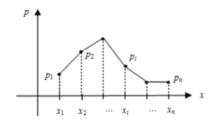
Operations on discrete probabilities
Distribution function
X
–28
–20
–12
–4
p
0,22
0,44
0,17
0,1
0,07
X
p
0,1
0,2
0,3
0,4
For binomial distribution M(X)=np, for Poisson distribution M(X)=λ
For binomial distribution D(X)=npq, for Poisson distribution D(X)=λExamples of solving problems on the topic “The law of distribution of a discrete random variable”
Task 1.
Task 3.
P 3 (0) = C 3 0 p 0 q 3-0 = q 3 = 0.9 3 = 0.729;
P 3 (1) = C 3 1 p 1 q 3-1 = 3*0.1*0.9 2 = 0.243;
P 3 (2) = C 3 2 p 2 q 3-2 = 3*0.1 2 *0.9 = 0.027;
P 3 (3) = C 3 3 p 3 q 3-3 = p 3 =0.1 3 = 0.001;
Check: ∑p i = 0.729+0.243+0.027+0.001=1.
for 0< x ≤1 имеем F(x) = Р(Х<1) = Р(Х = 0) = 0,729;
for 1< x ≤ 2 F(x) = Р(Х<2) = Р(Х=0) + Р(Х=1) =0,729+ 0,243 = 0,972;
for 2< x ≤ 3 F(x) = Р(Х<3) = Р(Х = 0) + Р(Х = 1) + Р(Х = 2) = 0,972+0,027 = 0,999;
for x > 3 there will be F(x) = 1, because the event is reliable. 
- mathematical expectation M(X) = np = 3*0.1 = 0.3;
- variance D(X) = npq = 3*0.1*0.9 = 0.27;
- standard deviation σ(X) = √D(X) = √0.27 ≈ 0.52.